
FisherPlot.jl: plotting your Fisher posterior contours
FisherPlot.jl is my first registered Julia package. It can be used to easily plot Fisher matrix contours, obtaining publication-quality results. In the remainder of this post, I'll give a (short) introduction to Fisher matrices, before showing how to use the package.
Fisher Matrix
You have an experiment that is going to collect some data and you want to understand how precisely you are going to measure some parameters Maybe you don't have collected any data, started your experiment or even obtained the money to build the experiment. Which error can we expect on the parameters we care about? Is there any correlation between our parameters? How much precision will you gain by buying a finer piece of equipment? Which numbers are you gonna put in that grant proposal? Performing a Fisher forecast can help you answer these questions.
In order to compute the Fisher matrix, you just need to know the likelihood of your data given the model parameters, , and compute minus the Hassian matrix of the log likelihood, :[1][2]
Once the Fisher matrix has been computed, the parameters covariance matrix can be easily obtained inverting the Fisher Matrix
Once you have computed the covariance matrix, the error on the -th parameter of the model is given by
But we have not finished yet: we can also obtain the correlation between the model parameters. Let us focus on the marginalized posterior of two parameters, namely and . The posterior is represented by an ellipse, whose semi-axes are given by:
while the ellipse orientation is given by
atan function not the ratio of the two elements in Equation (6), but the numerator and the denominator separately. If you are not going to do it, it is possible that the ellipse will be oriented in the wrong way!If you want a more detailed introduction to Fisher matrices, please refer to Coe (2009) and/or Heavens (2009).
FisherPlot.jl
In order to make our plots, we need some covariance matrices. Rather than creating some mock covariance matrices, I prefer to use some real-world matrices that I have calculated by myself[3]. In particular, I am going to use some covariance matrices calculated with my code CosmoCentral.
We are going to use three covariance matrices, each of them considering as observables the tomographic angular power spectrum 's coming from the following cosmological probes:
Weak Lensing
Photometric Galaxy Clustering
the combination of the previous two, plus their cross-correlation (usually known as )
These covariance matrices are computed following the approach of the Euclid official forecasts[4].
The parameters described by these matrices are the Dark Energy equation of state parameters[5][6], and , and the sum of the neutrino masses, .
C_WL = [0.0193749   -0.0620328  -0.00296159; -0.0620328    0.225214    0.0119904;
       -0.00296159   0.0119904   0.043537]
C_GC = [0.0150589   -0.0561336    0.00109151; -0.0561336    0.215808    -0.00562308;
        0.00109151  -0.00562308   0.00219601]
C_3x2_pt = [0.000724956  -0.00241439   0.000119474; -0.00241439   0.00844342   -0.000546318;
            0.000119474  -0.000546318   0.00113283]
Now we have to import a couple of packages, FisherPlot and LaTeXStrings
using FisherPlot
using LaTeXStrings
Now we need to define a few arrays, containing:
the name of the model parameters
the name of each covariance matrix
the color of each covariance matrix
LaTeXArray = [L"w_0", L"w_a", L"M_\nu\,[\mathrm{eV}]"]
probes = [L"\mathrm{WL}", L"\mathrm{GC}_\mathrm{ph}",
L"\mathrm{WL}\,+\,\mathrm{GC}_\mathrm{ph}\,+\,\mathrm{XC}"]
colors = ["deepskyblue3", "darkorange1", "green",]
Now we need to define a dictionary containing some objects needed by the plotter
PlotPars = Dict("sidesquare" => 600,
"dimticklabel" => 50,
"parslabelsize" => 80,
"textsize" => 40,
"PPmaxlabelsize" => 60,
"font" => "Dejavu Sans",
"xticklabelrotation" => π/4)
We are almost there! We now need to set up the central values for each parameter, the plot ranges and where we want to put the tick labels. This is something that you should take care of. For instance, we know that the sum of the neutrino masses is positive, so we want to avoid plotting the posterior for negative masses. In this particular case, we are going to use the Weak Lensing errors in order to decide the plot ranges.
central_values = [-1., 0., 0.06]

limits = zeros(3,2)
ticks = zeros(3,2)
for i in 1:3
    limits[i,1] = -4sqrt(C_WL[i,i])+central_values[i]
    limits[i,2] = +4sqrt(C_WL[i,i])+central_values[i]
    ticks[i,1]  = -3sqrt(C_WL[i,i])+central_values[i]
    ticks[i,2]  = +3sqrt(C_WL[i,i])+central_values[i]
end
limits[3,1] = 0
Finally, we need to prepare a white canvas and paint the contours on top of each other.
canvas = FisherPlot.preparecanvas(LaTeXArray, limits, ticks, probes, colors, PlotPars::Dict)
FisherPlot.paintcorrmatrix!(canvas, central_values, C_WL, "deepskyblue3")
FisherPlot.paintcorrmatrix!(canvas, central_values, C_GC, "darkorange1")
FisherPlot.paintcorrmatrix!(canvas, central_values, C_3x2_pt, "green")
Now, we can see the result! 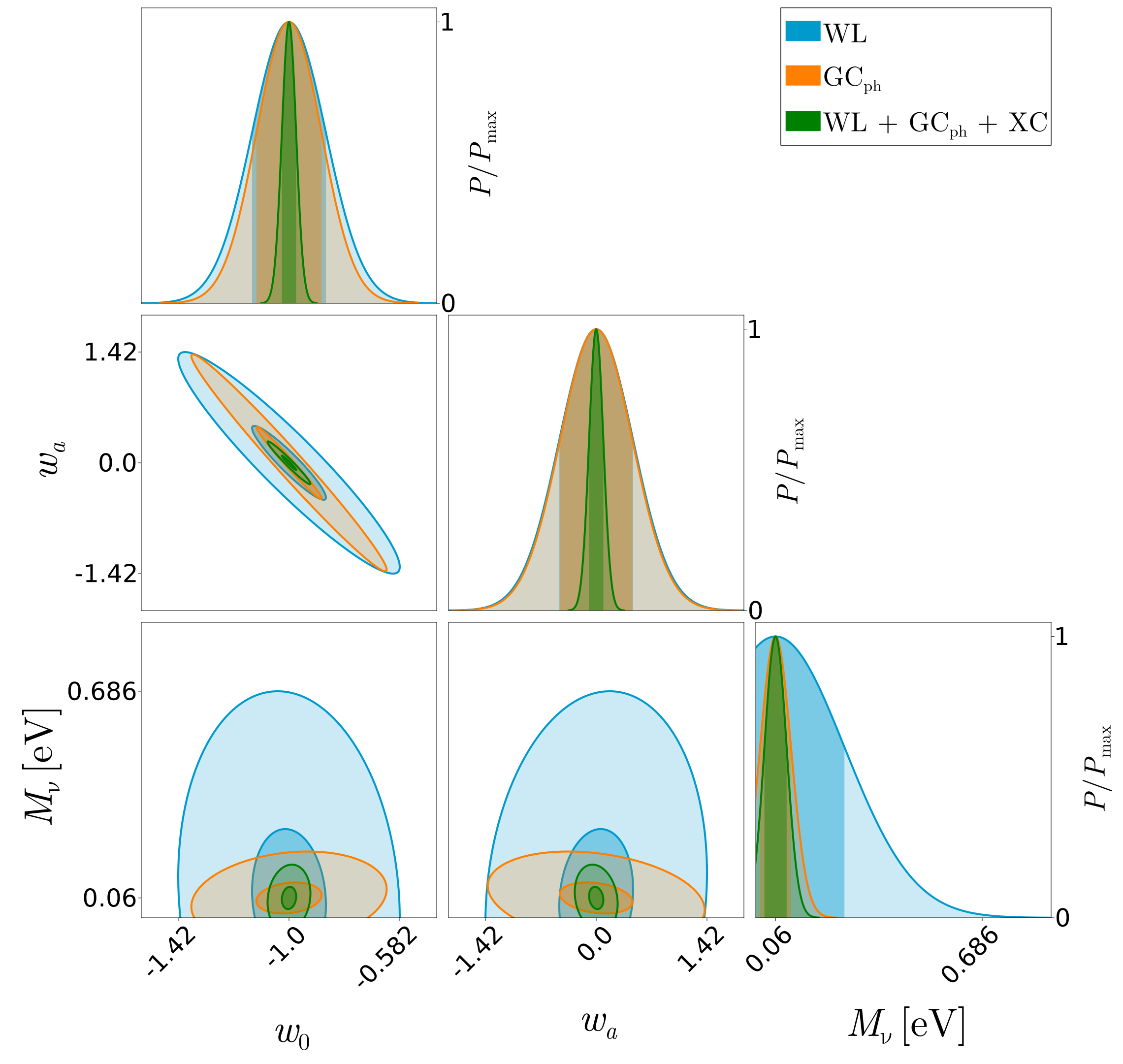
Quite nice, isn't it?
References & Footnotes
| [1] | Fisher, The logic of inductive science, Journal of the Royal Statistical Society (1935) |
| [2] | You can actually work out an analytical expression for your Fisher matrix, which is feasible for most cases, or use modern tools such as Automatic Differentiation and directly obtain the Hessian Matrix. |
| [3] | I mean: I am a scientist, and scientists are selfish. |
| [4] | Euclid Collaboration, VII. Forecast validation for Euclid cosmological probes, Astronomy & Astrophysics (2020) |
| [5] | M. Chevallier, D. Polarski, Accelerating Universe with scaling Dark Matter, International Journal of Modern Physics D (2001) |
| [6] | E. V. Linder, Exploring the Expansion History of the Universe, Physical Review Letter (2003) |